Category Archives: Atmospheric Physics

Cloudy feedback on global warming

Lawrence Livermore National Laboratory researchers have identified a mechanism that causes low clouds – and their influence on Earth’s energy balance – to respond differently to global warming depending on their spatial pattern.

The results imply that studies relying solely on recent observed trends are likely to underestimate how much Earth will warm due to increased carbon dioxide. The research appears in the Oct. 31 edition of the journal,Nature Geosciences.

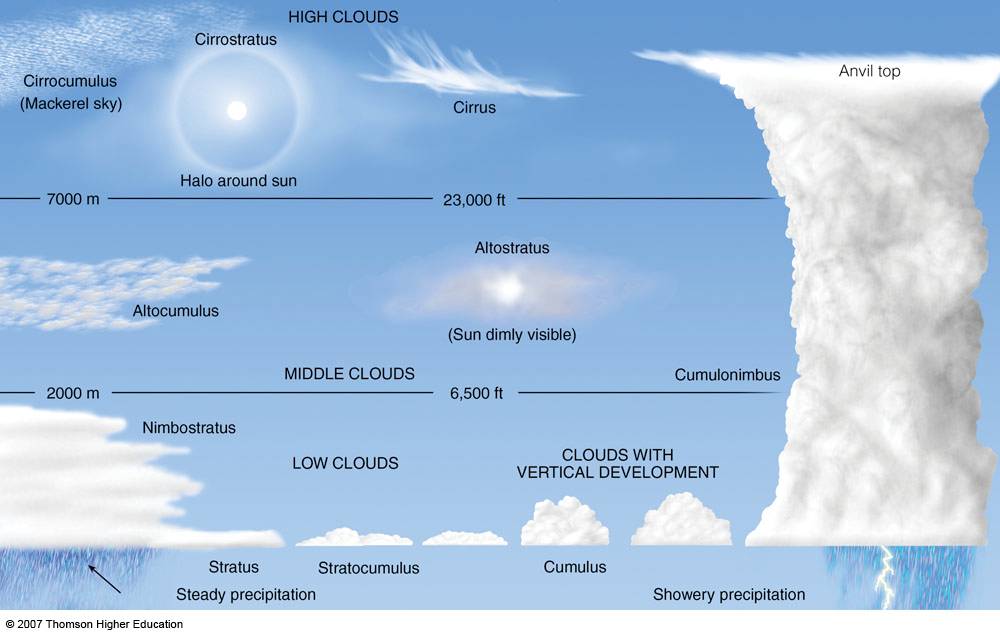
The research focused on clouds, which influence Earth’s climate by reflecting incoming solar radiation and reducing outgoing thermal radiation. As the Earth’s surface warms, the net radiative effect of clouds also changes, contributing a feedback to the climate system. If these cloud changes enhance the radiative cooling of the Earth, they act as a negative, dampening feedback on warming. Otherwise, they act as a positive, amplifying feedback on warming. The amount of global warming due to increased carbon dioxide is critically dependent on the sign and magnitude of the cloud feedback, making it an area of intense research.

This is an area attracting a great deal of research. The ramifications of changes in solar energy reaching the biosphere of earth could be serious. But studies reveal disagreement between a number of authors.

OCTOBER 31, 2016

Chen Zhou et al, Impact of decadal cloud variations on the Earth’s energy budget,Nature Geoscience (2016). DOI: 10.1038/ngeo2828

Cloud Cover and Global Warming

Experts reveal that clouds have moderated warming triggered by climate change.

A new study has revealed how clouds are modifying the warming created by human-caused climate change in some parts of the world.Led by Swansea University’s Tree Ring Research Group, researchers from Sweden, Finland and Norway analysed information contained in the rings of ancient pine trees from northern Scandinavia to reveal how clouds have reduced the impact of natural phases of warmth in the past and are doing so again now to moderate the warming caused by anthropogenic climate change.

The study, Cloud Cover Feedback Moderates Fennoscandian Summer Temperature Changes Over the Past 1,000 Years, is published in Geophysical Research Letters.

https://phys.org/news/2019-03-experts-reveal-clouds-moderated-triggered.html

Cloud-loss-could-add-8-degrees-to-global-warming

A recent article in Quanta Magazine reports that simulations indicate some cloud species may not form, causing a positive feedback in global warming, giving rise to added global temperature rise.

https://www.quantamagazine.org/cloud-loss-could-add-8-degrees-to-global-warming-20190225/

Ceilometers vs MPL

There is a decision to be made when deciding between these 2 forms of instrument when considering a monitoring program.

Firstly both Ceilometers and MPL ( Micro pulsed Lidar) are instruments based on the LIDAR principle. MPL uses photon counting detectors, while Ceilometers use avalanche photodiodes in analog mode. Beyond that all sampling and data conversion are digital.

Cost

Ceilometers are significantly lower in cost than MPL This is mainly due to the laser technology used. The lasers in Ceilometers can last up to 6-8 years and the laser replacement cost is relatively low.

Laser Pulse Source.

Most Ceilometers use a low cost solid-state pulsed laser diode, while the MPL uses a frequency doubled NdYag laser.

Wavelength

Most Ceilometers emit in the range 905 to 920 nm, which is not visible and the launch pulses are reduced in energy so that the sensor is eye safe. The MPL emits at 532 nm and is able to launch higher energy pulses meaning the range is greater, or conversely the ability to detect low levels of scattering ( eg MIE ) at low levels is enhanced. Potential users need to look at the differences between scattering properties of the target at the 2 wavelengths.

Polarisation

Ceilometers do not have dual polarisation channels and the discrimination capabilities of MPL may make them more suitable for the planned studies

Deployment Costs

Ceilometers are designed to be operated long term in a wide range of environments and are more suited to remote deployment where there is less maintenance available.

Ceilometers are widely used for PBL studies. Because of increased range/sensitivity MPL is favoured in high cloud studies, but high range ceilometers are available and might be selected if a multi sensor long term study is being undertaken.

Ceilometers for Cloud Amount

A recent paper by Wagner and Kleiss compares a Ceilometer with Total Sky Imager and Micropulse lidar looking at suitability of ceilometers for estimation of cloud amount.

https://journals.ametsoc.org/doi/pdf/10.1175/JTECH-D-15-0258.1

In summary they say, in part:

“Ceilometers will be a mainstay of the operational automated weather observation network for years to come.

They are relatively inexpensive and require little ongoing maintenance, and are capable of 24-h observations.
While TSIs produce automated observations that are qualitatively more similar to human observations of sky cover than the ceilometer, ongoing operational
costs like mirror cleaning and reduced hours of operation limit this instrument’s applicability for deployment in unattended environments.

Two significant sources of error are associated with the automated sky cover observations obtained by single ceilometer ASOS installations: the spot view of the instrument renders it unable to see the entire sky, while the 3660-m height limit renders the instrument incapable of observing high clouds. These errors are not insignificant, and their magnitudes vary depending on the actual cloud coverage. The spatiotemporal averaging error is smallest for clear and overcast conditions as the sky exhibits little variability in these conditions. The high cloud error is at its smallest when skies are dominated by low clouds, and it tends to increase as low cloud coverage lessens, allowing high clouds to peek through.”

The ability to reliably detect upper atmosphere cloud is restricted to a subset of available ceilometers which have ranges in excess of the usual 7,500 to 10,000 metre range. Such ceilometers include the a CL51, the 8600-CHS and the CHM15K

ToPROF: Ceilometers and Lidar Applications

As part of the EU “COST” programmes, the ToPROF group is working on operational ground based profiling with ceilometers, doppler lidars and microwave radiometers for improving weather forecasts.

Work started in 2014, and is progressing towards a nominal completion date in 2020.

For overall details refer to the ToPROF Home Page

Within the To PROF group, a Ceilometer Working group has been established.

Here are the details of this working group This group would be of interest to those within the following End-Users

National weather services (incl. COPERNICUS/MACC): calibrated attenuated
backscatter profiles to evaluate NWP models (through forward operators); Cloud
base height for NWP evaluation and weather monitoring.
Agencies in charge of atmospheric surveillance for air traffic: occurrence, height and mass concentrations of ash layers; diagnostic and short-term forecast of fog and other low visibility events.
Agencies in charge of Air Quality monitoring: boundary layer height; freetropospheric aerosol transport.
Networks in charge of GHG monitoring: boundary layer height to quantify GHG
dilution effects.
EUMETSAT: European-wide validation of cloud-base height and fog
Renewable energy industry: Photovoltaic ReN – cloud/fog fraction and evolution for nowcasting applications (combined with geostationary satellite); Concentrated solar power: aerosol vertical distribution; Wind ReN – wind profiles from Doppler Lidars.

International Commission on Clouds and Precipitation (ICCP)

The International Commission on Clouds and Precipitation (ICCP) is a Commission of the International Association of Meteorology and Atmospheric Sciences (IAMAS)
The IAMAS is one of the associations of the International Union of Geodesy and Geophysics (IUGG)

The ICCP holds a conference every 4 years. The last conference was at Manchester University in 2016, The next is due in 2020.

Typical subjects in calls for papers are theoretical, observational and numerical modelling studies of cloud and precipitation physics, cloud chemistry and cloud dynamics.

For instance the following subjects are commonly covered at the conferences

Basic cloud and precipitation physics
Warm boundary layer clouds
Convective clouds (including cloud electrification)
Mixed phase clouds (including Arctic/Antarctic stratus, mid-level clouds)
Cirrus clouds
Orographic clouds
Fog and fog layers
Mesoscale cloud systems (including severe storms)
Tropical clouds
Southern Ocean clouds
Polar stratospheric clouds and noctilucent clouds
Aerosol-cloud-precipitation-interactions and processing
Clouds and climate (including radiative properties of clouds)
Ice nuclei and cloud condensation nuclei
Cloud and precipitation chemistry
Measurement techniques (of cloud and precipitation properties) and uncertainties
Applications of cloud and precipitation physics

New WMO Cloud Atlas

The WMO has released a new Cloud Atlas. The release was timed to coincide with the World Meteorological day. 23/3/2017

Here is the Press Release

Here is the Home page for the new Cloud Atlas.

Ceilometers and Snow

Like Rain, Snow produces quite high levels of backscatter. But the raindrops and snow flakes have very different shapes, velocities and surface area to mass ratios. More expensive ceilometers may have the ability to discriminate between snow and rain.

A typical LIDAR curtain plot for cloud appears below:

snow plot

Ref: University of Utah Atmospheric Science

The snow is coming from a cloud at around 500m . The cloud and snow appear to extinguish the returns from higher layers, if any. Some of the snow is light and evaporates before it gets to ground level. ( low level green return )

Work has been done to try to determine snowfall rate from Lidar returns. According to Ed Eloranta of the University of Wisconsin Madison, the technique requires radar and does not require any knowledge of the snowflake shape.

Download Poster

Click to access arm_09.pdf

Ceilometers for Dust Storm Profiling

Sydney Dust Storm 2009

A wall of dust stretched from northern Queensland to the southern tip of eastern Australia on the morning of September 23, 2009, The storm, the worst in 70 years, led to cancelled or delayed flights, traffic problems, and health issues, The concentration of particles in the air reached 15,000 micrograms per cubic meter in New South Wales during the storm, A normal day sees a particle concentration 10-20 micrograms per cubic meter.

Work on the use of Ceilometers for analysis of that Dust Storm is decribed in the paper:

Laser ceilometer measurements of Australian dust storm highlight need for reassessment of atmospheric dust plume loads By Hamish McGowan and Joshua Soderholm

Among the more interesting information in this paper was the curtain plot showing the increase in backscatter when the wall of the duststorm hit, the very high concentration around ground level and the vertical extent of the dust. The maximum vertical extent of this plot is 1500 metres , or approx 5000 ft.

(Curtain Plot showing onset of the Dust Storm and estimated particle Concentration from paper: Laser ceilometer measurements of Australian dust storm highlight need for reassessment of atmospheric dust plume loads By Hamish McGowan and Joshua Soderholm )

Ceilometers like the 8200-CHS are suitable for this type of work, where dust storms are experienced regularly, such as the Harmattan in sub saharan Africa, the Churgui in Morocco, the Khamasin in Egypt, the Shamal in Iraq or the Kali Andhi in India

High Altitude Clouds

High Altitude clouds fall into 2 categories,

Those with a low base and vertical development are Cumulonimbus and Towering Cumulus. At the base these are water clouds, so the ceilometer only “sees” a few hundred feet into the cloud.
Those with a high base, including Cirrus, Cirrostratus and Cirrocumulus and Altostratus

The Cirrus cloud family are composed of Ice Crystals, and are very often “optically thin”and they have low backscatter coefficients, so are difficult to detect with ceilometers, because the laser pulse energy is limited to eye safe levels.

Altostratus may be composed of ice crystals. In some ice crystal altostratus, very thin, rapidly disappearing horizontal sheets of water droplets appear at random. The sizes of the ice crystals in the cloud tended to increase as altitude decreased. However, close to the bottom of the cloud, the particles decreased in size again

Altostratus cloud with a water phase may have a strong backscatter signal and can be picked up as in the case below

17000 FT 26-11 TREVISO

Alto stratus Cloud at 17,000 ft

Ref 1 : Wikipedia : Alto Stratus entry.

Ref 2. Wikipedia Cirrus Cloud entry.

Cloud Atlas

The definitive reference to cloud types and Cloud species is the ICAO Cloud Atlas which can be downloaded for free from this site:

WMO Cloud Atlas Vol 1 WMO Cloud Atlas Vol 2

There are a number of less detailed cloud type images on the internet. For example

The Australian Bureau of Meteorology have a good references to cloud observation

Australian Bureau Chapter 13

Cloud Types Graphic

Current ceilometers have a range out to about 25,000 ft, and other models with larger telescopes built in,. can reach up to about 40000 ft. For use in aviation, at airports a range of 12,00 ft is considered adequate.

Sky Condition, How is it assessed ?

A human observer looks at the sky and estimates the coverage in 8ths , 0 being clear sky and 8 being overcast. The human observer then estimates cloud height and applies these estimates of cover for each layer. It is quite obvious that if there are no breaks in the sky, any higher layers present cannot be estimated. The human observer also suffers from the “packing” effect of an oblique line of sight , and usually tends to overestimate cover.

For each layer the human observer will give the condition FEW, SCATTER, BROKEN AND overcast.

A ceilometer can only “see” cloud above it, so can only estimate the sky condition by analysing heights over a time period.

The Sky Condition Algorithm in the 8200-CHS is based on that developed by the US National Weather Service and used in their automated surface observing system (ASOS) units and guidelines published by the World Meteorological Organization.

A study by the Hughes STX Corp. found that when ceilings were under 5,000 feet, this algorithm agreed with the human observer 78% of the time. With fog, the comparability was 84%, with rain it was 69%, and when snowing 74%. During rain, the NWS Algorithm reported more changes than the human observer.

However at the transition between scattered and broken cloud coverage 4 oktas humans often report too much cloud coverage. This is attributed to the “packing effect;” a condition where an observer does not see the openings in the cloud decks near the horizon due to the viewing angle. Pilots tend to overestimate the coverage even more than ground observers because of visual compression.

The 8200-CHS algorithm is not biased by the “packing effect” because it measures only the sky conditions passing over the sensor

Details of the 8200-CHS specifications can be found here 8200-CHS Page

Why tilt a ceilometer?

A slight tilting of the ceilometer gives better performance in rain.

Rain drops tend to flatten as they fall. See the NASA explanation for this

Consequently, when aligned vertically the backscatter from raindrops may be sufficiently high to cause difficult in resolving the cloud base above the rain.

However when tilted, the backscatter of laser pulses by the raindrops is reduced .

In heavy rain even a tilted ceilometer cannot resolve the cloud base since the integrated backscatter quickly dominates and prevents further penetration up to the cloudbase, while extinction in the return path also starts to extinguish the return signal..

Please refer to the screen below.

These tests were carried out during light rain. The tilted unit shows resolvable cloud base while the untilted unit reverts to vertical visibility.

Cloud Appreciation Society

The Cloud Appreciation Society has some great cloud Photos and covers a lot of information about clouds from all over the world.

Cloud Appreciation Society

Here is one of the really good photos .

Cloud Appreciation Society : A classic Cumulonimbus with an arcus feature on the leading edge, spotted near Pipestone, Minnesota, US. © Edward Carberry

Cloud Types: Cumulo Nimbus and AltoStratus

Stratus clouds, irrespective of altitude have a more or less constant and solid base , indicating stable layers in the atmosphere and lack of thermal activity.

By contrast the Cumulo Nimbus cloud betrays a high degree of vertical motion of the atmosphere and thermal activity. Cumulus congestus and Towering cumulus display a moderate degree of vertical extent

In the curtain plot below, the classic rapid change of cloud level characteristic of Cb cloud can be seen between 19.00 and 23.00 hours. After that time the cloud base solidifies and rises to 6500 ft

Cb cloud gives way to As cloud

Cb cloud gives way to Ac cloud

Calibrating a Ceilometer

There are 2 types of calibration.

Calibrating the distance measurement: In this case the ceilometer is turned on its side and aimed at a hard target. In this case the ceilometer is aimed at a tree 4450 ft away. The exact distance of the tree was surveyed using Google Earth. The ceilometer was aimed using a telescopic sight. The backscatter profile is an almost perfect replica of the laser pulse, delayed by the time taken for the laser pulse to go to the target and back.

8200-CHS HARD TARGET AT 4450

In reality, the calibration of the ceilometer is based on the well known speed of light and if the timing crystal inside the ceilometer is accurate and stable, the distance calibration is stable and accurate and should never need to be checked in the service life of the ceilometer.

Clouds are not solid reflectors, and the backscatter comes from a range of scatterers inside the cloud, so the backscattered laser pulse is broadened and flattened. The height of the cloud is defined as a threshold in the backscatter profile which has been determined will result in a correct reading for most types of cloud.

2. Calibrating the ceilometer constant. For this , there is a clever method as described in a paper by O’connor et al, which utilises the known Lidar Ratio of 18.8 in stratocumulus cloud ( SC).

A technique for autocalibration of cloud lidar

8200-CHS Ceilometer multi level clouds

The 8200-CHS has the capability of detecting up to 4 simultaneous layers but certain types of standard messages display only 3 layers .

If the lowest layer is optically dense, the returns from beyond the first layer are extinguished , and the layers above it are not detected until a gap in the lower layer is detected. If the cloud is not optically dense, the return from a higher level cloud is not significantly attenuated when passing back through the lower layer, so both layers can be detected.

Here is a case where multiple layers are at 6620 and 7290 are both detected.

: Clouds at 6620 and 7290 ft